Constraint forces for path in 3D

This is a post mostly for my future self. What got me thinking about it was this comment about my planetary tunnels post:

Straight tunnels? What about ones using the Lagrangian drooping rope optimized as the line?

— Andrew Jagger (@ajagger01) February 27, 2023

which is actually referring to a really old post of mine about how to dig a well.

In order to add in the effects of a spinning planet, there are two or three major routes I could take:

1. Set the constraints on the path to be for a spinning path.
2. Just add the coriolis and centrifugal forces to my other calculations
3. Do either (1) or (2) with some Lagrange Multipliers so that we could interrogate the constraint forces keeping the ball on in the tunnel

This post is really about (3), though I’ve done (2) and it’s pretty cool. I just put in the fictitious forces, but only those components that are along the tunnel (using a dot product). Here’s the result:

What constraints do we use for the Lagrange Multiplier approach?

When you do Lagrange Multipliers, which you usually do because you want to learn something about the forces that enforce the constraint, you need to have a formula of something that (typically) stays constant for all the dynamics.

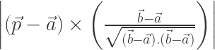
I first thought I could do this with a single constraint. I figured if we have points a and b on the line and we want to find a measure of how far a third point, p, is form the line, we’d get a distance and the constraint would be that the distance should always be zero. I can get that distance by asking for the length of the vector given by crossing a normalized vector on the line with the vector from the point of interest, p, to either end point. As I tell my students, when you use a cross product, one vector is saying to the other: “hey you, how much of you is perpendicular to me?” and that perpendicular distance is exactly what I’m looking for. So, I figured this would work for a constraint (it should be zero for any point on the line):

So I tried it! Holy crow, it’s slow in the Wolfram Engine (Mathematica for free). Actually, if I start the simulation on the line, the WE just gives up:

r[t_]:={x[t],y[t],z[t]};
constraint=Cross[r[t]-p1,p2-p1].Cross[r[t]-p1,p2-p1];
KE=1/2 r'[t].r'[t];
PE=4/3 Pi r[t].r[t];
L=KE-PE;
el[a_]:=D[L,a[t]]-D[L,a'[t],t]+lm[t] D[constraint,a[t]]==0;
sol=First[NDSolve[{el/@{x,y,z},
                   x[0]==p1[[1]],
                   y[0]==p1[[2]],
                   z[0]==p1[[3]],
                   x'[0]==0,
                   y'[0]==0,
                   z'[0]==0,
                   D[constraint,t,t]==0},{x,y,z,lm},{t,0,1}]]

NDSolve::ndcf: Repeated convergence test failure at t == 0.; unable to continue.

If I start it just off the line, it meanders up and down the line, maintaining its distance. But, wow, it’s a really slow integration (note: all I did was change the x[0] value to p1[[1]]+0.01 on line 8)

Here’s a plot of the constraint function (note that it stays pretty constant):

Since it was so slow, I wanted to find another way. That’s when I realized that a straight line is given by the intersection of two planes. So maybe I could just say “hey, it’s on this plane and on that plane at all times.” That’s equivalent to saying that we have two constraints, not just the one like above.

So how do you find the equations for a plane (or two for that matter) that the original line is on? Well, the formula for a plane is so we just need to find two sets of a, b, c, and d that do the trick. What I did was:

Solve[{a x1+b y1+c z1+d==0, a x2+b y2+c z2+d==0}, {a,b,c,d}]
{{c -> -((a*(x1 - x2))/(z1 - z2)) - (b*(y1 - y2))/(z1 - z2), 
d -> -((a*(x2*z1 - x1*z2))/(z1 - z2)) - (b*(y2*z1 - y1*z2))/(z1 - z2)}}

and the WE told me the relationships you have among them. Then I just arbitrarily chose two sets of a and b (<0,1> and <1,0>) and calculated two sets of c and d. Then I just used those two equations in the Solve command as my (2!) constraints and it worked. And it was really fast.

c[a_,b_]:=0. + 0.3998911137852679*a - 0.2628716901520667*b;
d[a_,b_]:=0. + 0.9517484637723629*a - 0.5145497461933767*b;
r[t_]:={x[t],y[t],z[t]};
c1={0,1,c[0,1]}.r[t]+d[0,1];
c2={1,0,c[1,0]}.r[t]+d[1,0];
KE=1/2 r'[t].r'[t];
PE=4/3 Pi r[t].r[t];
L=KE-PE;
el[a_]:=D[L,a[t]]-D[L,a'[t],t]+lm1[t] D[c1,a[t]]+lm2[t] D[c2,a[t]]==0;
sol=First[NDSolve[{el/@{x,y,z},
                   x[0]==p1[[1]],
                   y[0]==p1[[2]],
                   z[0]==p1[[3]],
                   x'[0]==0,
                   y'[0]==0,
                   z'[0]==0,
                   D[c1,t,t]==0,
                   D[c2,t,t]==0},{x,y,z,lm1,lm2},{t,0,1}]]

What about non-straight line?

A general path in 3D can be given by three parametric equations where you use a fourth variable to connect them all:

• x=f(t)
• y=g(t)
• z=h(t)

That looks like three constraints but when using Lagrange Multipliers you don’t really want to have that extra variable (t in this case). You want to only use x, y, and z and have extra unknown force terms that the ODE solver solves for.

So really you have to invert one of those 3 equations. Often one of them is amazingly simple, like f(t)=t. If that’s true, then you have two constraints:

• y-g(x)
• z-h(x)

and you’re off and running!

Here’s an example where g(x) is sin(x) and h(x) is cos(x). This is a helical path:

c1=y[t]-Sin[x[t]];
c2=z[t]-Cos[x[t]];
r[t_]:={x[t],y[t],z[t]};
KE=1/2 r'[t].r'[t];
PE=-9.8 x[t];
L=KE-PE;
el[a_]:=D[L,a[t]]-D[L,a'[t],t]+lm1[t] D[c1,a[t]]+lm2[t] D[c2,a[t]]==0;
sol=First[NDSolve[{el/@{x,y,z},
                   x[0]==0,
                   y[0]==0,
                   z[0]==1,
                   x'[0]==0,
                   y'[0]==0,
                   z'[0]==0,
                   D[c1,t,t]==0,
                   D[c2,t,t]==0},{x,y,z,lm1,lm2},{t,0,3}]]

Producing this path:

Note that I put in a potential energy in all of these examples. I could have just set that to zero, but then to get things to move I’d have to set the initial velocity. For the straight lines, that’s relatively easy, but for the helix I’d have to think carefully about what direction it starts moving in. So much easier to start things at rest and let a (conservative) force take over.

Your thoughts?

I’d love to hear your thoughts. Here are some starters for you:

• This is super helpful. What I especially like is . . .
• This is dumb. I hope future you realizes that.
• This is future you. Thanks for this, it’s really come in handy.
• This is future you, watch out for that thing tomorrow.
• Really? You’re going to start using WE instead of “the mathematica kernel you can use for free”? That seems too informal.
• I’m still not sure I get why you insisted on adding a potential energy to all these examples.
• Why do you use for the potential energy in a planet?
• What do you mean by a conservative force? What’s wrong with a liberal force?