Rigid bodies, formulation and examples

My friend Rhett Allain gave me a good challenge recently with this tweet:

What about a bead on a freely rotating hoop that can rotate in three dimensions?
— Rhett Allain (@rjallain) November 23, 2022

I had been working on a problem that he posted about regarding a bead sliding freely on a hoop that is spinning about an axis in its plane that goes through the center. That’s a pretty typical Lagrangian Dynamics-type problem and I wondered what would happen if the hoop wasn’t driven to constantly go with a particular angular frequency but rather was set spinning on that axis with that initial angular frequency but after that it would respond dynamically (speed up or slow down its rate of spinning) according to the physics involved. Here’s what that looks like:

But then when Rhett asked about letting the hoop be even more free to rotate, in other words not just around that one axis, I realized I’d have to calculate things a different way.

That led me to remind myself how to do Lagrangian Dynamics with rigid bodies, mostly dealing with things like the Inertia Tensor and body axes. This post is to make it so I don’t have to start from scratch with that again. Note that this post lays out the broad strokes of what I’m doing here.

Lagrangian dynamics with rigid bodies

For those of you hoping I’ll derive the Euler rotation equations, I should let you know that I don’t explicitly do that here. I get close, but I really move in a direction where I can solve the equations of motion and make some fun vids of the motion.

Here’s the steps involved:

Determine the generalized coordinates
Determine the kinetic and potential energies
Use the Principal Axes (actually you don’t have to do that)
Do all the usual Lagrangian stuff

Generalized coordinates (Euler rotations)

If you need to describe the orientation of a rigid body, how would you do it? I’ve done this with my students by asking them to all grab their chairs and figure out a systematic way to orient them the way mine is (which I do when they have their eyes closed). At first students think you just need the polar angles $\theta$ and $\phi$ because they figure that all the r’s are fixed and so you don’t need that third polar coordinate. But then I show them two situations with my chair that share the polar angles but look different. Ultimately my students usually land on a version of the Euler angles, which are really just the polar angles with a final twist of the body around the original vertical axis. Most texts call that last angle $\psi$ .

Well, if the Euler angles are the information that you need to describe the orientation of a rigid body, that means they’re just the perfect generalized coordinates for a Lagrangian Dynamics approach. All we have to be able to do is describe the potential and kinetic energy of the object as functions of the Euler angles and we’re good to go!

Kinetic and Potential energy as functions of the Euler angles

Early on physics students learn that if they’re dealing with rotating bodies they can replace $\frac{1}{2} m v^2$ with $\frac{1}{2} I \omega^2$ . Essentially what happens is that you realize that all parts of the system share an angular speed ( $\omega$ ) even if different parts are traveling with different linear speeds (v). Since they all share the same thing, you can pull that out of any sums or integrals you’re doing to add up all the kinetic energy and whatever’s left you just lump into something we call the moment of inertia ( $I$ ).

The problem is that for oddly shaped things that simple approach doesn’t quite work. Sure all the pieces and parts still share an angular velocity (now we’re talking about the vector $\vec{\omega}$ since the axis of rotation is something we need to know), but it’s not as simple as $\frac{1}{2} I \omega^2$ . Probably the easiest way to see that is that the angular momentum is not necessarily parallel to the angular velocity (STOP: read that again, as it’s one of the single most important aspects of rigid body motion and it sounds really weird to most people). Instead there’s a relationship between the angular momentum vector and the angular velocity vector that’s more complicated. If you know the angular velocity you can find the angular momentum with a 3D rotation, and that’s done computationally with a 3×3 tensor which we call the inertia tensor. Then you have $\vec{L}=\overleftrightarrow I\cdot\vec{\omega}$ . Essentially a 3×3 tensor dotted into a vector gives you a new vector that (often) points in a new direction (hence them not being parallel anymore).

Really the inertia tensor has just what we need. Just like we can do $\frac{1}{2}\vec{p}\cdot\vec{v}$ for kinetic energy normally (try it!), we can do $\frac{1}{2}\vec{L}\cdot\vec{\omega}$ or:

$\text{Kinetic Energy}=\frac{1}{2}\left(\overleftrightarrow I \cdot \vec{\omega}\right) \cdot\vec{\omega}$

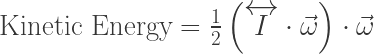
Aha! So now if we know how both the inertia tensor and the angular velocity vector can be described by the Euler angles (and their time derivatives) we’re in business!

The inertia tensor is certainly calculate-able if you know the orientation of the object (which you do if you know the Euler angles). Essentially you can figure out where all the particles of the body are and then do all the integrals necessary for the inertia tensor (remember, the tensor is just made up of what’s left after you factor out the common terms that all the particles share – namely the angular velocity – so it’s just a collection of sums/integrals involving the locations of the particles). What really sucks, though, is that at every point in time there is a new orientation and hence a whole new set of integrals to do. Ugh. Don’t worry though, that gets a lot easier in the next section!

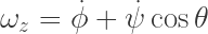
The angular velocity is certainly a function of the time derivatives of the Euler angles since as they change they rotate the body, and rotation is all that angular velocity is used to describe. Here’s the cool part: the angular velocity ( $\vec{\omega}$ ) is equal to the sum of three vectors, one for each Euler angle. Each Euler angle contributes it’s time derivative (which is exactly the right units for angular velocity) in the direction of the instantaneous axis of rotation that Euler angle rotates around. I know, that was complicated, but it’s relatively straightforward to work out:

First consider the easiest one: $\phi$ . When you think about it that polar vector, all it does is rotate everything around the vertical-, or z-, axis. Therefore $\phi$ ‘s contribution to $\vec{\omega}$ is $\dot{\phi} \langle 0, 0, 1\rangle$ .

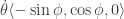
Next consider $\theta$ : When it changes, it tilts the object further from the vertical. But it does so in the plane determined by $\phi$ . The instantaneous axis of rotation is the location of the new y-axis after the $\phi$ rotation. So that means that the $\theta$ contribution to $\vec{\omega}$ is $\dot{\theta}\langle -\sin\phi,\cos\phi,0\rangle$

Finally we have $\psi$ . It rotates the body around its original vertical axis. That means its instantaneous axis of rotation is wherever its vertical axis has gotten to after the polar angles have done their thing. So $\psi$ ‘s contribution is $\dot{\psi}\langle \sin\theta\cos\phi, \sin\theta\sin\phi,\cos\theta\rangle$ .

All together then we have these for the components of the angular velocity vector:

$\omega_x=-\dot{\theta}\sin\phi+\dot{\psi}\sin\theta\cos\phi$

$\omega_y=\dot{\theta}\cos\phi+\dot{\psi}\sin\theta\sin\phi$

$\omega_z=\dot{\phi}+\dot{\psi}\cos\theta$

Only calculate the inertia tensor once!

Ok, we have the angular velocity all set to go, but we saw how the inertia tensor, while definitely a function of the Euler angles, might have to be calculated over and over again. What if we only had to do it once!

The trick is to decide to think about how things feel in the frame of the rigid body. In what we call the “body-frame” it sits there while the world moves around it. Specifically the angular velocity vector is all over the place. But, and this is the important part, the inertia tensor is fixed! You just have to calculate it once in that orientation. So the problem becomes determining what the angular velocity vector (which we calculated above) looks like in that body-frame.

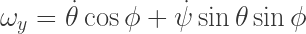
But luckily the Euler angles were built to transform any vector into a new rotated state. So we just need to apply the Euler rules to the angular velocity vector above. Except that we’re trying to describe how things look to the body frame, so what we really need is the reverse of the Euler rules, namely:

negative rotation of $\phi$ around the z-axis, followed by. . .
a negative rotation of $\theta$ around the y-zaxis, followed by . . .
a negative rotation of $\psi$ around the z-axis

I know, that seems weird, but, trust me, it does the trick. All of those rotations are pretty straightforward for something like Mathematica to do so we’re in business: Calculate the inertia tensor once, figure out the lab-based angular velocity vector, and then do the steps above to find the body-frame version of the angular velocity vector. Then you calculate the kinetic energy.

Here’s what that looks like in Mathematica:

After the “KE=…” line is the usual construction of how I do Lagrangian Mechanics. The “Method->…” stuff was suggested by Mathematica after the first solve seemed to fail. That Method fix did the trick.

You’ll note that my inertia tensor (“Ithing”) is really simple. There are no off-diagonal terms in the matrix because I wanted to investigate the same sort of thing I did in this post about flipping handles in space. The section below called “Principal Axes frame” is how I teach my students to find the magical orientiation of an object where its inertia tensor has that simple setup. Note that it’s not necessary for the work I’ve laid out here.

Note that while this makes it pretty do-able, you’re still going to want a Computer Algebra System to help. Here’s just the $\theta$ Euler-Lagrange equation (all of this equals zero) for a generic inertia tensor:

Putting it to use to answer Rhett

Ok, so now I had the tools to answer Rhett’s question. I’ve got an interesting system made up of a hoop and a bead. What I decided to do was to fix $\psi$ for the hoop at zero because otherwise I would have to keep track of the bead’s sliding separate from the rotation of the hoop around it’s (original) vertical axis. The orientation of the hoop when all the Euler angles are zero is horizontal. So I first set $\theta$ to $\pi/2$ to stand it up and then I set $\dot{\phi}$ to some initial spin rate.

For the bead I just determine it’s contribution to the inertia tensor of the system. Luckily that’s just a simple function of $\psi$ (remember I fix that at zero for the hoop). So I basically do the same thing as before. Here’s the Mathematica:

Really I have to carefully do the hoop and the bead separately when doing the $\omega$ calculations, but otherwise it’s similar to what I did above.

Here’s the results!

You can see how the hoop starts to tilt over. It has to to maintain a constant angular momentum (since there’s no torque in the problem if you don’t fix the axis of the hoop).

Principal Axes frame

I noted above that you don’t have to use the principal axes frame but I wanted to put this in for my future self:

When I teach this I point out how difficult things are when the angular moment is not parallel to the angular velocity. I ask them if they’d like it if we could make that disappear. Usually they say yes.

I tell them that there are some magic scenarios when the two are parallel. Essentially there are three axes that if you rotate around them you get an angular momentum in that same direction. There are a few ways to figure them out, but most are either difficult to understand mathematically (eigenvectors of the inertia tensor) or would take forever (just spin the object along all possible axes and look to see when the angular momentum is along that same axis). But there’s one way I’ve found that my students can do. I have to explain how a diagonalized inertia tensor does the trick. I do that by saying that we’ll just keep orienting the object until we find that all three of the magic axes are along the normal lab axes (x-, y-, and z-axes). In that orientation, you get what we need as long as there are no non-zero off-diagonal components of the inertia tensor.

So I provide my students with a Mathematica document that lets them freely adjust the Euler angles for an object and it constantly recalculates the inertia tensor for that orientation (see the last section above to understand why the tensor changes with orientation). What’s cool is that they can see how certain adjustments to the Euler angles tends to reduce at least one of the 3 off-diagonal components and they usually quickly find a systematic way to get them all to be vanishingly small. When they do that, they’re staring at the orientation that puts the magic axes along the lab axes!

Your thoughts?

I’d love to hear what you think. Here are some starters for you:

I love this! What I especially am surprised by is . . .
This is dumb. I especially hated . . .
So whatever Rhett says you just do? That sounds interesting . . .
Once again no python, loser
I thought you only had a chromebook at home. How are you doing all this Mathematica?
Whoa, it looks like you do the $\psi$ rotation first in your Mathematica code. Didn’t you say it comes last?
Wait, I don’t have to diagonalize the inertia tensor before doing these kinds of simulations? That’s so cool!
Do you provide tools to help your students unbolt their chairs from the desks?
I want to hear more about how students can systematically find the principal axes by just adjusting the Euler angles!
Why don’t you have to do the normal accelerated frame adjustments for your kinetic energy? (it’s quite late as I type this and I realize I don’t have a good answer beyond “it just works”)