AppSheet ideas

AppSheet is a google product that enables you to use Google Sheets as a backend database for a mobile app that works in both the Android and Apple ecosystems. I encourage you to check it out, as it’s become a go-to tool for me to think about interacting with students and my colleagues at my school. Quick note: it’s really designed to be used by people on the same domain (yourcoolschool.edu, for example), not really to produce a true mobile app for the world. This post is about some brainstorming I’ve been doing to think about a campus app that could be useful.

What I’ve done so far

Here’s a quick list of the apps I’ve built and some of the cool features they make use of:

• Hamline Go
  • This is an app I built to try to help build community on campus. Students can see faculty and staff avatars on a map and collect them by clicking on them. They get one point for every collection unless its a faculty member who teaches in their major, then it’s 5 points. If instead they actually talk to a faculty or staff member and get their hourly code, they get 10 points. Certain offices on campus also have hourly codes. I also built in flash (1 hour), daily, and weekly challenges like “write a haiku about your major” or “prove you found this spot on campus”. Point leaders after the end of each month get declining balance (money) prizes.
  • Tools used:
    • Google Maps
    • Login features (checks user email and crosschecks the faculty in their declared major)
    • Editable images (you can draw on images before submitting them for the challenges)
    • Google Apps Script running independently to update both the avatar locations (randomized on our campus) and the hourly codes
• Majors t-shirts
  • Every major program was encouraged to design a tshirt that we would then order for any declared major that wanted one. I built an app to show students the designs available to them (only the designs for their declared majors) and let them submit the size that they wanted.
  • Tools used:
    • Login (check their major and crosscheck against the submitted designs)
    • Selfie collection (students are encouraged to submit a selfie wearing their tshirts so we can make a collage)
• Scavenger hunt
  • I made an app that encourages first year students to learn about the various offices on campus. Each campus had a QR code displayed that, if the students scanned it using the app, indicated that the student had visited that office
  • Tools used
    • QR code reader
    • Login

I’ve made it quite a bit up the learning curve, including some of these really useful tips and tricks:

• Make a slice of the users data called “me”. Have it be a filter of all the users that match the useremail() (a built in function). Essentially it’s a data source with just one row in it. Then I use index(me[id], 1) to get the current user’s id when doing a lot of the crosschecking mentioned above. I do the same thing on any of the related collections. In Hamline Go, for example, I make a “my avatars” slice to show the avatars that have been collected by that user. Then I can send that slice as the core data to a “view” that shows avatars.
• Use an automation to send a notification whenever there’s a new flash challenge. They only last an hour, so it’s helpful to let the students know there’s a new one. These notifications come as push notifications to the students phones.
• Pre-fill forms using LinkToForm that can take a collection of values to pre-fill elements. You can also then not show those elements in the form view and so it looks magical!
• Send email notifications to people that include live forms right in gmail. This works really great for approvals.

What I’m hoping to do

I’d love to create an app that I’m currently calling “Hamline All Around”. Here are some of the features I hope to build in:

• Somehow provide a navigation aid through our various systems. We get a lot of feedback from students who say they just don’t understand how to accomplish various things, especially the ones that are supposed to be providing valuable resources to them. A great example is our emergency grant program.
  • One thing I’m thinking of is a dynamic FAQ that might ask what sort of thing they’d like to accomplish and then quickly get them to the office they should start with.
• “Find a study buddy!” I gather other schools do this and so I built a quick test to see if this would work. The student logs in and it shows them the classes they’re taking. For each they can “raise their hand.” If they do, they see all the other students who’ve done the same, all of whom are indicating that they’re interested in finding study buddies. They can see each other’s emails, or potentially use the app’s push notification system to communicate. I also made a form that lets them say “I plan to study tomorrow night in the library from 7-8” and the others who’ve raised their hands can indicate if they plan to come. This is displayed in a nice calendar format that looks a lot like google calendar.
• Show the student group and athletic team calendar events in one place (right now you have to separately subscribe to both ical streams, but appsheet can do the subscription and display them in the app)
• Event check in: All employees and students have bar codes on the back of their ids and appsheet can read them (it’s a setting for one of the built-in form elements). It would be very easy to build in an event check-in system where the event runners (multiple of them) could have the app running on their phones and they could scan in the students/staff/faculty who attend. Once they do, the app on the students/staff/faculty phones could become much more functional (ie the app, upon being updated, would detect that the person is checked in and would then show all the relevant functionality for the event).
• Directions: Often it’s not enough to tell people what building things are in. Directions for how to actually get to the office can come in handy. I’ve been wondering about vids showing someone literally walking from a common place to an office, all the while describing what useful things the office can do for students.

Help!

I’m excited to work on this, but I’d love some more brainstorming, including poking some of these ideas a little. Here are some starters for you:

• I love this. What I especially love is . . .
• This is dumb. What I especially dislike is . . .
• Wait, you’re tracking the location of all faculty and staff in real time?! (note: it took me a long time to convince people I wasn’t doing that. I call the things avatars and try to make it clear that I just randomly place them on the campus map. However, several faculty and staff were deeply suspicious of this app and asked to be taken out of the app.)
• I think the “find a study buddy” app is really interesting. Have you thought about . . .
• I think the “find a study buddy” app is really disturbing. Instead you should . . .
• So after you figure out all the views and the data connections you have to learn how to write it for both the Android and iOS systems?! (no! Appsheet does all that for me. All the students have to install is Appsheet which already exists in both ecosystems)
• We’ve got a student app on our campus and I love it. Here are my favorite parts . . .
• We’ve got a student app on our campus and I hate it. What would make it so much better is . . .
• Here’s some additional functionality you should think of . . .
• Can you please do some tutorials on how to do all this in Appsheet?
• What’s an example of a haiku about a major?
  • Minnesota Law
  • Ins and Outs of Policing
  • Criminal Justice

Constraint forces for path in 3D

This is a post mostly for my future self. What got me thinking about it was this comment about my planetary tunnels post:

Straight tunnels? What about ones using the Lagrangian drooping rope optimized as the line?

— Andrew Jagger (@ajagger01) February 27, 2023

which is actually referring to a really old post of mine about how to dig a well.

In order to add in the effects of a spinning planet, there are two or three major routes I could take:

1. Set the constraints on the path to be for a spinning path.
2. Just add the coriolis and centrifugal forces to my other calculations
3. Do either (1) or (2) with some Lagrange Multipliers so that we could interrogate the constraint forces keeping the ball on in the tunnel

This post is really about (3), though I’ve done (2) and it’s pretty cool. I just put in the fictitious forces, but only those components that are along the tunnel (using a dot product). Here’s the result:

What constraints do we use for the Lagrange Multiplier approach?

When you do Lagrange Multipliers, which you usually do because you want to learn something about the forces that enforce the constraint, you need to have a formula of something that (typically) stays constant for all the dynamics.

I first thought I could do this with a single constraint. I figured if we have points a and b on the line and we want to find a measure of how far a third point, p, is form the line, we’d get a distance and the constraint would be that the distance should always be zero. I can get that distance by asking for the length of the vector given by crossing a normalized vector on the line with the vector from the point of interest, p, to either end point. As I tell my students, when you use a cross product, one vector is saying to the other: “hey you, how much of you is perpendicular to me?” and that perpendicular distance is exactly what I’m looking for. So, I figured this would work for a constraint (it should be zero for any point on the line):

So I tried it! Holy crow, it’s slow in the Wolfram Engine (Mathematica for free). Actually, if I start the simulation on the line, the WE just gives up:

r[t_]:={x[t],y[t],z[t]};
constraint=Cross[r[t]-p1,p2-p1].Cross[r[t]-p1,p2-p1];
KE=1/2 r'[t].r'[t];
PE=4/3 Pi r[t].r[t];
L=KE-PE;
el[a_]:=D[L,a[t]]-D[L,a'[t],t]+lm[t] D[constraint,a[t]]==0;
sol=First[NDSolve[{el/@{x,y,z},
                   x[0]==p1[[1]],
                   y[0]==p1[[2]],
                   z[0]==p1[[3]],
                   x'[0]==0,
                   y'[0]==0,
                   z'[0]==0,
                   D[constraint,t,t]==0},{x,y,z,lm},{t,0,1}]]

NDSolve::ndcf: Repeated convergence test failure at t == 0.; unable to continue.

If I start it just off the line, it meanders up and down the line, maintaining its distance. But, wow, it’s a really slow integration (note: all I did was change the x[0] value to p1[[1]]+0.01 on line 8)

Here’s a plot of the constraint function (note that it stays pretty constant):

Since it was so slow, I wanted to find another way. That’s when I realized that a straight line is given by the intersection of two planes. So maybe I could just say “hey, it’s on this plane and on that plane at all times.” That’s equivalent to saying that we have two constraints, not just the one like above.

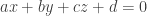So how do you find the equations for a plane (or two for that matter) that the original line is on? Well, the formula for a plane is so we just need to find two sets of a, b, c, and d that do the trick. What I did was:

Solve[{a x1+b y1+c z1+d==0, a x2+b y2+c z2+d==0}, {a,b,c,d}]
{{c -> -((a*(x1 - x2))/(z1 - z2)) - (b*(y1 - y2))/(z1 - z2), 
d -> -((a*(x2*z1 - x1*z2))/(z1 - z2)) - (b*(y2*z1 - y1*z2))/(z1 - z2)}}

and the WE told me the relationships you have among them. Then I just arbitrarily chose two sets of a and b (<0,1> and <1,0>) and calculated two sets of c and d. Then I just used those two equations in the Solve command as my (2!) constraints and it worked. And it was really fast.

c[a_,b_]:=0. + 0.3998911137852679*a - 0.2628716901520667*b;
d[a_,b_]:=0. + 0.9517484637723629*a - 0.5145497461933767*b;
r[t_]:={x[t],y[t],z[t]};
c1={0,1,c[0,1]}.r[t]+d[0,1];
c2={1,0,c[1,0]}.r[t]+d[1,0];
KE=1/2 r'[t].r'[t];
PE=4/3 Pi r[t].r[t];
L=KE-PE;
el[a_]:=D[L,a[t]]-D[L,a'[t],t]+lm1[t] D[c1,a[t]]+lm2[t] D[c2,a[t]]==0;
sol=First[NDSolve[{el/@{x,y,z},
                   x[0]==p1[[1]],
                   y[0]==p1[[2]],
                   z[0]==p1[[3]],
                   x'[0]==0,
                   y'[0]==0,
                   z'[0]==0,
                   D[c1,t,t]==0,
                   D[c2,t,t]==0},{x,y,z,lm1,lm2},{t,0,1}]]

What about non-straight line?

A general path in 3D can be given by three parametric equations where you use a fourth variable to connect them all:

• x=f(t)
• y=g(t)
• z=h(t)

That looks like three constraints but when using Lagrange Multipliers you don’t really want to have that extra variable (t in this case). You want to only use x, y, and z and have extra unknown force terms that the ODE solver solves for.

So really you have to invert one of those 3 equations. Often one of them is amazingly simple, like f(t)=t. If that’s true, then you have two constraints:

• y-g(x)
• z-h(x)

and you’re off and running!

Here’s an example where g(x) is sin(x) and h(x) is cos(x). This is a helical path:

c1=y[t]-Sin[x[t]];
c2=z[t]-Cos[x[t]];
r[t_]:={x[t],y[t],z[t]};
KE=1/2 r'[t].r'[t];
PE=-9.8 x[t];
L=KE-PE;
el[a_]:=D[L,a[t]]-D[L,a'[t],t]+lm1[t] D[c1,a[t]]+lm2[t] D[c2,a[t]]==0;
sol=First[NDSolve[{el/@{x,y,z},
                   x[0]==0,
                   y[0]==0,
                   z[0]==1,
                   x'[0]==0,
                   y'[0]==0,
                   z'[0]==0,
                   D[c1,t,t]==0,
                   D[c2,t,t]==0},{x,y,z,lm1,lm2},{t,0,3}]]

Producing this path:

Note that I put in a potential energy in all of these examples. I could have just set that to zero, but then to get things to move I’d have to set the initial velocity. For the straight lines, that’s relatively easy, but for the helix I’d have to think carefully about what direction it starts moving in. So much easier to start things at rest and let a (conservative) force take over.

Your thoughts?

I’d love to hear your thoughts. Here are some starters for you:

• This is super helpful. What I especially like is . . .
• This is dumb. I hope future you realizes that.
• This is future you. Thanks for this, it’s really come in handy.
• This is future you, watch out for that thing tomorrow.
• Really? You’re going to start using WE instead of “the mathematica kernel you can use for free”? That seems too informal.
• I’m still not sure I get why you insisted on adding a potential energy to all these examples.
• Why do you use for the potential energy in a planet?
• What do you mean by a conservative force? What’s wrong with a liberal force?

Does the hoop hop?

I greatly enjoyed this recent video from StandUpMaths:

The set up is a hoop with a mass attached at one point. It’s rough so it rolls without slipping. It’s released with some angular momentum with the extra mass starting at the top. The question is whether the hoop loses contact with the ground as it rolls around. The original analysis from decades ago focused on a mass-less hoop and suggested that the hoop has to hop when the mass has rolled around just 90 degrees.

I wanted to see what it would take to model this. What I thought would be useful would be to use a Lagrange Multiplier technique so that I could easily check the normal force on the ground, watching to see if it ever goes to zero, as that’s when it would hop. If the normal force goes negative, that means the ground is pulling the hoop down. And the ground doesn’t usually do that.

Math/physics setup

When you use Lagrange Multipliers, you tend to have more degrees of freedom in the problem. In fact you have the normal number of degrees of freedom (one in this case: $latex \theta) plus however many constraints you model with Lagrange Multipliers. I want to model both the normal force and the rolling-without-slipping force. For the normal force, my constraint is:

where r is the radius of the hoop and y is the y-component of the center of the hoop.

For the rolling-without-slipping constraint I use:

where x is the x-component of the center of the hoop and is the rotation angle. When the mass is at the top.

The kinetic energy is given by:

Where we treat the center of mass of the hoop as one free particle and the mass as another. Note, however, that we stipulate that the location of the mass is tied to the location of the center:

Then we just do the usual Euler Lagrange tricks and we’re off and running.

m=1;
mhoop=0;
r=1;
g=9.8;
omega=0.1;
xm[t_]:=x[t]+r Sin[th[t]];
ym[t_]:=y[t]+r Cos[th[t]];
KE=1/2 m (xm'[t]^2+ym'[t]^2)+1/2 mhoop (x'[t]^2+y'[t]^2)+1/2 (mhoop r^2) th'[t]^2;
PE=m g ym[t]+mhoop g y[t];
rollingConstraint=x[t]-r th[t];
normalConstraint=y[t]-r;
L=KE-PE;
el[a_]:=D[L,a[t]]-D[L,a'[t],t]+lmRolling[t] D[rollingConstraint,a[t]]+lmNormal[t] D[normalConstraint,a[t]]==0;
sol=First[NDSolve[{el/@{x,y,th},
          x[0]==0,
          y[0]==r,
          th[0]==0,
          x'[0]==r omega,
          y'[0]==0,
          th'[0]==omega,
          D[rollingConstraint,t,t]==0,
          D[normalConstraint,t,t]==0,
          WhenEvent[lmNormal[t]==0,"StopIntegration"]},{x,y,th,lmNormal,lmRolling},{t,0,10}]];
tmax=sol[[1,2,1,1,2]]

The “WhenEvent” trick stops the integration right at the point of when the hoop would hop. I don’t always use that, you’ll see, in my animations below.

Results

Here’s a plot of the normal force for the case of a truly massless hoop:

You see that it starts at 9.8 because the mass is 1kg and the ground is really just holding the hoop+mass up (remember that the hoop is massless). It’s not actually exactly 9.8, though, since right at the beginning there’s a non-zero angular speed, , and so the some of the gravity force needs to be dedicated to centripetal acceleration.

Here’s an animation that stops right at the point of hopping:

Now lets give the hoop just a little bit of mass: 0.01kg (so 100x less than the attached mass). Here’s a normal force plot showing that I allowed the simulation to go past the hopping point. Note that I don’t let it hop. Rather, I allow the normal force to go negative.

Here’s an animation of that setup:

Finally let’s consider a situation where the mass of the hoop equals the mass of the attached point. Here’s a normal force plot:

Note that it never goes to zero. Here’s an animation:

Cool, huh?

Your thoughts?

I’d love to hear what you think. Here are some starters for you:

• This is cool! What I liked the most was . . .
• This is dumb! What you totally got wrong was . . .
• Wait, I thought you saw this on a math(s) youtube channel. This seems like physics.
• I don’t think that mass is undergoing circular motion, so saying that some of the gravity is providing a centripetal force doesn’t seem right.
• I suppose you’re not going to bother posting your code, are you?
• I can’t believe you insist on using a super expensive software package like Mathematica . . . wait, what did you say 3 posts ago?
• That youtube video talks about looking at when the hoop starts to slip. Couldn’t you do that by looking at your rolling Lagrange Multiplier and seeing if it gets larger than the expected friction?

Planetary tunnel oscillators

Pick a point on the earth and start digging. It doesn’t have to be straight down. Keep it straight (careful! it’s harder than you might think) and keep going until you come back to the surface. Ok, now drop a ball into your hole. It’ll come back to you eventually because while gravity will pull it down the hole at the beginning, eventually it’ll start getting further from the center of the earth and start slowing down. Assuming the earth’s density is spherically symmetric, it’ll come to a stop right at the edge of the other end, turn around, and come back.

If in addition to being spherically symmetric the earth’s density was also uniform, the travel time of the ball will be independent of the direction you dug the hole. In other words connect any two points on the surface of this idealized earth and the time it takes the ball to tunnel from one point to the other and back will be the same! Pretty cool, right?

I wanted to see if I could 1) make cool animations of that, and 2) see if my intuition would be right for non-uniform spherically symmetric densities. Before you scroll any further, make a prediction: If the planet is more dense towards the center, will a tunnel that gets close to the center take more or less time than a shallow tunnel?

The model

I modeled this using the Wolfram Engine (for free!) which is basically mathematica but using a Jupyter interface. I used a Lagrangian approach which just means I needed to identify the degrees of freedom (the distance down the tunnel) and figure out how to express both the kinetic and potential energy for a particle using that variable. If p1 and p2 are the two points on the surface of the earth, I parametrized my problem with the variable s such that if s is zero we’re at p1 and if s is one we’re at p2. When s is between zero and one it’s in the tunnel:

Then the kinetic energy is:

which will be a function of s.

The potential energy is a little trickier but basically it’ll always be:

where the total Mass, M, that is closer to the center that the point of interest is given by:

assuming r is less than the radius of the planet.

Simulations

Here’s a plot of s as a function of time for a uniform density planet in a universe where G=1, m=1, and the radius of the planet = 1:

Here’s an animation of 10 different random tunnels all dug from the north pole. Note how they stay in sync:

Ok, time to check your intuition. Consider a planet whose density varies as 1/r. That means it’s technically infinitely dense right at the center and it progressively gets less dense as you get further out. Which tunnels will be faster? The ones that are shallow, and so only ever experience the lower densities, which means they always feel nearly the full gravitational pull of the planet? Or the ones that dive deep and explore portions of the planet with high densities?

Here’s what I was thinking: The shallow ones never penetrate where the bulk of the mass is. That means their force stays high. Therefore I think they should be faster.

Here’s a plot of 10 random tunnels, note how they don’t stay in sync:

Here’s the animation:

For me it’s easiest to see the effect if you stare at the upper left purple one and keep your peripheral attention on the central green one. You can tell that the shorter path takes longer! I was wrong!

Ok, what about the opposite: a density that grows linearly with distance from the center. That means there’s no density at the center and the maximum density is at the outer edge.

First a plot of the trajectories:

and here’s the animation:

See how the lower right red one really falls behind? Cool, huh?

Your thoughts?

I’d love to hear what you think about all this. Here are some starters for you:

• This is really cool! What about a planet that . . .?
• This is really dumb! What you forgot about was . . .?
• My intuition was right! Here’s what I was thinking . . .
• My intuition was wrong! Therefore all of physics is wrong.
• I just assume the potential energy is always GMm/r and you just have to figure out the M. (that’s what I naively thought too as I started but realized that you have to do the integrations to get it right)
• Did you set all the planets to have the same total mass? (yes)
• Why do you insist on using an expensive piece of software that normal people can’t afford . . . wait, what did you do two posts ago?
• What happens if the density is not spherically symmetric? What are you, lazy?
• You clearly didn’t model the effects of a spinning planet, even though you forced us to click through to a whole other blog post about digging holes. Be consistent!
• Why didn’t you dig identical tunnels for all three planets? It’s super tough for me to directly compare them. My guess is you got all excited about using RandomPoint[Sphere[], n] in the Wolfram Engine.

Dropping ladders

My friend Rhett Allain has really got me interested in this ladder drop posted by Veritasium:

Here’s Rhett’s awesome explanation:

Of course I wanted to see if I could model it with Mathematica, and, after finding I could run Mathematica for free on my windows laptop, I thought I’d revisit this problem, since I think I found something interesting.

Physics involved

Here’s what I did:

• I modeled the rungs of the ladder as rigid sticks with a mass, a length, and moment of inertia
• I modeled the ground as a one-way spring (it only pushes up if either end of the rung goes below the ground, it doesn’t pull back down when either end is above the ground)
• I modeled the strings holding the rungs together as one-way spring as well. If they stretch, they pull. If they’re compressed, they do nothing.
• I modeled frictional energy loss by treating the ground as a viscous fluid. Any time either end is under the ground, there’s a frictional force proportional to the speed of that end that is in the opposite direction of the motion. Here’s a youtube vid I made about that approach.

I did all of that in a Lagrangian formalism. The one-way springs are piecewise potential energy functions, for example.

I had to play around with the strength of the ground one-way spring to make sure the bounces seemed realistic and also with the amount of viscous friction so that the rungs came to a stop relatively quickly.

What it looks like

Here’s an animated gif showing 4 very similar ladders. From left to right:

• Moment of inertia of each rung is
• Moment of inertia of each rung is
• Moment of inertia of each rung is
• Free fall (doesn’t hit the ground so the moment of inertia doesn’t matter)

Here’s a plot (along with a zoomed-in inset) of the height of the middle of the top rung for each of those ladders:

You can see that the smaller the moment of inertia of the rung, the faster it falls.

Using Rhett’s explanation (which I really think is right), when a tilted (that’s important!) rung hits the ground, it slaps down the other end, which stretches the string tied to that end, which then pulls down, at least slightly, on the rung above it. This continues in a domino like fashion. Ultimately all that “pulling down” is what accelerates the top rung faster than free-fall.

The differences for the moment of inertia is what I find interesting. The one is a rung that has a uniform cross-section (ie, the mass is uniformly spread through the length). The one is what you get if all the mass of the rung is at the ends. Really this is the highest possible moment of inertia for a rung. The lowest possible is zero if all the mass is in a point mass at the center, but for fun I did to see a more obvious effect. With a higher moment of inertia, the “slaps down” effect I talk about above is lessened, because the rung is harder to rotate. That means the “pulls down” effect is lessened as well and so you see that there’s less additional acceleration for the top rung. In the plot above you can see that the maximum moment of inertia is indistinguishable from free-fall.

Your thoughts

I’d love to hear what you think. Here’s some starters for you:

• I love this! I’m going to build a minimal moment of inertia ladder right now.
• This is dumb. What you totally missed in your model was . . .
• I don’t know why you insist on using such an expensive tool like Mathematica . . . wait, what did you say in your last post?
• I don’t like your friction model. Instead I think you should . . .
• I think your rungs are bouncing too high, you should raise your friction amount. (I did that but found that it reduces the “slap down” too as it doesn’t just cause rotation, it also moves the end a little bit. Something to think about, I guess)
• I think all ladder rungs are uniform. This is stupid.
• I think Veritasium doctored that first video. There’s no way there’s two ladders with every rung angle being exactly the same.
• Hang on a sec, it looks like you’ve pinned the center of the rungs on a vertical line. That’s crap and you know it.
• Are you saying that if all the rungs are perfectly horizontal nothing happens? How boring.

Mathematica for free

In this post I’m going to try to capture the steps I took today to get a Jupyter Notebook to run Mathematica commands. I did it on a Windows laptop so if you’re on a Mac of Linux you’ll have to make appropriate adjustments.

Why free?

Mathematica is not free. A single license can be over $1000. Student versions are more like $200 but there’s no question that it’s pricey, especially when compared with python-based computing. Of course, it definitely has value! The amount of development that’s been poured into it, including just in the last few years, is amazing. Want easy to use neural networks? Check. Want lightning fast prototyping? Check. Want access to tons of curated data sets that all play well together? Check.

But, ugh, what a cost. And it’s hard to convince students to embrace it if they know they’ll lose it as soon as they graduate. I’ve spent lots of time looking for a replacement for the types of things I tend to work on, and it’s been a mixed bag.

But ever since I noticed that Wolfram (the company that makes Mathematica) put a free mathematica kernel (what they now call a Wolfram Engine) on the Raspberry Pis, I started keeping an eye out for ways to use the Wolfram Engine for free.

If you go here you’ll see that you can download the engine for developers and use it for free as long as you’re not trying to make money with it. When you download it and install it you can then run wolframscript in a cmd window and you get old-school command-line Mathematica. Graphics don’t work but general calculations do.

To get a more useful interface, you can pair it with a Jupyter Notebook. These are free interfaces that people mostly use to do Python programming. But you can swap out the kernel from Python to Wolfram Engine with the steps that I outline below.

So the kernel (Wolfram Engine) is free (assuming you’re not trying to make money) and Jupyter Notebooks are free. Off we go!

Installation steps on Windows

1. Download and install the Wolfram Engine
   • You’ll have to register on their site (for free) to get it to work.
   • Run wolframscript in a cmd window and it’ll ask for your login credentials for Wolfram.
2. Install python
   • Note, I couldn’t get this to work with Anaconda, so I uninstalled Anaconda and separately installed python, pip, and jupyter
3. Install pip
   • Go to “Method 2” on this page
   • Make sure to install it in the same folder where python is.
     • To figure that out, run py on the cmd line and run this code:

>>> import os
>>> import sys
>>> os.path.dirname(sys.executable)

4. Install Jupyter
   • in that same directory, run this code: pip install jupyter
5. Download the paclet
   • Go to this website
   • Then go down to “Assets” and download the file called WolframLanguageForJupyter-x.y.z.paclet (for me x=0, y=9, z=3)
   • Make sure to save it to the same folder where python and pip are now installed
6. Run a few commands in command-line mathematica
   • In that directory, run the wolfram engine with this command: wolframscript
   • In Mathematica run these commands one at a time:
     • PacletInstall["WolframLanguageForJupyter-x.y.z.paclet"] (make sure to use the right x, y, and z)
     • Needs["WolframLanguageForJupyter`"] (note the extra back tick toward the end there)
     • ConfigureJupyter["Add"]

And you’re done! Now you just need to run jupyter by typing jupyter notebook on the command line and it should launch a new tab in your browser (it takes about a minute on my machine, it seems). Then you can select a new file using the Mathematica kernel:

Finally, here’s a youtube vid of me using it (showing how to model a 10-pendula)

Your thoughts?

I’d love to hear your thoughts. Here are some starters for you:

• This is cool! My favorite part is . . .
• This is dumb. The dumbest part is . . .
• Why don’t you italicize Mathematica?
• Can it do Manipulate commands? (sort of)
• Can it access the curated data? (haven’t tried yet)
• Why didn’t you do an 11-pendulum? Jerk
• I can do all this a lot easier with scipy, loser.
• Can you write this up for Mac users?

Computational Data Science capstone class

In just over a week the CDS capstone class starts and I’m not nearly ready. It’s been a while since I taught a class (Spring 2021 in the pandemic) and I’m a little rusty. But I remembered how useful it is to do syllabus planning on here so I thought I’d give it a try.

[Brief aside to explain why I find this useful: Making little notes to myself can work great, and I can use shorthand for all the things I want to get done. Doing it here forces me to spell everything out, and what I’ve found is that it gets me thinking more deeply about everything. I guess it’s the prospect of you, dear reader, paying attention and not wanting to embarrass myself in front of you, but it really works to get my thoughts more concrete. Plus there’s the added bonus of getting great feedback from you. Finally, when I read these things in future years it helps me to have all those details spelled out, as my cryptic notes tend not to make any sense years later.]

Class context

Our CDS major is pretty new, with only a few graduates so far. This will be the second time this class is taught, but I didn’t teach it last time. This class is typically for seniors in their last semester. It finishes up the major and it meets a couple important general education requirements (oral intensive class and independent learning class). The main goal of the class is to have the students complete a major project using a computational lens on their chosen area of focus. They are required to take at least three courses in that area of focus, with at least one at the intermediate level.

Here are details about the program and the major. The required classes include a python programming class, my Intro to CDS courses (which is a lot more python including web scraping and api managment), a couple stats courses, and a few courses borrowed from the Math (discrete math) and Business Analytics majors.

Organization

Last year the instructor treated each day of the week very differently and I really like the general structure:

• Mondays: hear from students about a particular data tool
• Wednesdays: specific support for their projects
• Fridays: Sample presentations on different data sets

Mondays (tool sharing)

There’s less than 10 students in the class (another reason I’m teaching it) so they’ll all be able to present at least one tool on Mondays. My hope is that we don’t get any repeats and we all develop a stronger tool set. One big question about those days is whether I should try to get them all to be in python, but I’m not sure how much I care about that. I’ll likely do the first day (8 days from now!) so I’ll need to think about what’s a good model.

Could more than one student go in a week? Should they get the whole class period? That’s a lot of pressure but they only have to do it roughly once. Maybe I could model the first few weeks before we really get it going.

I think it should be ~15 minutes of explaining what problems the tool helps with, ~15 minutes about the logistics of using it, ~15 minutes showing it off, and ~15 minutes brainstorming how people might make use of it.

Wednesdays (student project support)

These are the days where I’ll scaffold the work they’ll need to do to really get their projects going. Rather than saying “hey your big project is due at the end of the term, good luck!” I want to make sure that there are near-weekly benchmarks for them to achieve. We’ll not only have them due on those Wednesdays but we’ll make sure that those class times are filled with reflective activities.

My biggest challenge is getting them to be resources for each other, especially since likely no two students will have the same focus area.

Early in the semester we’ll spend time refining what the projects are. The idea of a computational lens on their focus area really needs to be tightly defined so that I’m not constantly making them change direction throughout the term.

Mid-semester will be about helping each other brainstorm deeper ideas, figuring out which things are important and which things are just showing off some tool.

Late semester will be all about refining the final product, namely a video presentation of their project.

Fridays (Data storytelling)

Each week I’ll give them a new data set on Monday. For each they have to come up with a 5-minute live presentation on Friday telling a story with that data. While this takes them away from their project (I likely won’t give them data they’re already working with) it helps them practice the work of computational storytelling and they get to see just how many diverse stories can be told.

One of my colleagues has a ton of useful data sets he’s letting me borrow. A lot of them have to do with the criminal justice system. I also plan to try to be flexible and use timely data that’s in the news. One example that I’m still thinking about is the list of school closings on the most recent snow day we had (last week). What would you do with that?

What else?

I really like that structure but there are some parts that need to be refined. For example, what exactly determines the grade in the class? I’m of course partial to a Standards-Based Grading approach, so let me flesh out what that would look like:

• A standard (or several) on how to share a tool
• A standard (or several) on how to learn about a new tool
• A standard (or several) on how to tell a story with a data set
• A standard for all the various parts of the scaffolding for the main projects

That last one, especially, is crap. If the project is a bunch of points, then the SBG approach means it doesn’t matter what they do during the scaffolding. I’ll need to think more about that.

Another approach is the contract- or specifications-grading where I lay out the expectations for A-level, B-level, etc work and they work at the pace/quality/etc they want to achieve. That works really well for a big project-based class so I’ll have to give that some thought over the next week as well.

The key, for me, with all of these types of decisions is finding a system that provides accountability and motivation for the students to learn as much as they can. That’s what I’ll be focusing on this week.

Your thoughts

I’d love to hear what you think. Here are some starters for you:

1. Why has it been so long since you taught? Surely you haven’t moved to the dark side.
2. Why didn’t you teach it last time? Did they know how much you’d stink at it?
3. Wait, your general education requirements are embedded in majors courses?
4. Why does the small class size explain why you’re teaching it?
5. Of course Mondays should be all python all the time, why would you even consider other things?
6. Here’s my definition of “computational lens on a focus area” . . .
7. I’m going to be in this class. I’m most excited about . . .
8. I’m supposed to be in this class. Now that I’ve read this, how do I drop?
9. I think it’s dumb to try to get them to help each other out on Wednesdays. Instead you should . . .
10. Here’s what I’d do with the school closing data . . .
11. You seriously haven’t decided which grading scheme to use yet? Loser.
12. Your plan for Mondays adds up to 60 minutes. Surely you actually only teach 50 minute classes!

Rolling without slipping on curved surfaces

I’ve been trying to see if I can model balls rolling on curved surfaces and I think I’ve cracked it. Here’s a teaser to get you interested:

What you see is a sphere rolling on a curved surface. The blue line is the path of the contact point and the orange line is the path of the center of the ball. What that ball is doing is called “rolling without slipping” which just means that the contact point doesn’t slide at all. In fact, the part of the ball in contact with the surface is (momentarily) at rest!

Rolling without slipping is something that happens in nature a lot. If something isn’t doing that (like a bowling ball at the beginning of your throw), it often is brought to rolling-without-slipping by friction. Once it gets to that point it tends to stay in that condition. So I thought it would be cool to learn how to model it.

So why did I think this would be an interesting challenge? It seems that introductory physics courses have problems with rolling without slipping all the time. It’s how we learn that rolling balls get down hills slower than the point mass calculations we typically start students with. The reason is that the potential energy of the hill has to be split between the translational kinetic energy that we think of with point particles *and* the rotational kinetic energy it gets while rolling. That’s why it’s slower.

But the reason this is interesting is I wanted to do two things: figure out the angular rotation at all times so that I could make fun animations, and ask what happens if you don’t just do a boring inclined plane — specifically a surface that’s curved.

2D first

First I tackled an effective 2D problem, or a problem I can draw on a sheet of paper. The easiest to do is a non-curved surface that’s at an angle. The rolling without slipping condition in that case is pretty easy:

where v is the speed of either the contact point (remember, the part of the ball touching the plane doesn’t move, where that point is does) or the speed of the center of the ball, since they’re the same if the surface is flat.

Now consider the Lagrangian approach for the problem. Let’s assume the angle the line makes with the horizontal is . Here’s my chicken scratch, barely legible approach:

If you like using x for horizontal and y for vertical, you use the first part. If you want to use a variable along the slope, you use the bottom part (where I used the variable “a”). Either way you get a pretty straightforward result showing that it moves down the slope at a constant acceleration that’s less than g, thanks to the rolling. Note that for the rest of this post I’ll be using the x and y approach because the slope is constantly changing making the “a” approach tricky.

Alright, so what happens when the surface is curved? I ran into this in my Brachistocrone for rolling things post, and the upshot is that the rolling without slipping condition changes to:

where is the speed of the contact point.

Here’s my notes where I proved that to myself:

The key it to realize that while the yellow and orange stripes line up as it rolls, the sphere is frustrated from fully executing its rotation because the curve has risen up to meet it. The part that’s taken back is that that’s labeled.

For that old post the more complicated expression was a major pain in the butt, and I was convinced for a few weeks it would be for this too until I went back to the paper I referenced in that post again a couple days ago and realized that you get a much cleaner version of the rolling without slipping condition:

which looks just like my simple one up at the top of this post! Yep, if you just switch to the speed of the center of the ball, instead of the speed of the contact point, you get to use our old tried-and-true rolling without slipping condition. This was the big breakthrough I needed!

Here’s the setup:

1. Choose the generalized coordinate as (the x-location of the contact point). Assume .
2. Find expressions for the coordinates and velocities of the center of the ball based on
3. Using the trick above for the rolling-without-slipping condition, determine the kinetic and potential energies of the ball, at first in terms of the center coordinates but ultimately in terms of
4. Do the usual Euler-Lagrange trick to find the equation of motion for
5. Give both the EOM (and the initial conditions) along with the rolling-without-slipping condition to the differential equation solver so that you can get both and as functions of time
6. Make fun animations

First let’s consider 1 & 2. Here’s an image showing most of the important variables:

How do you get the center-of-ball coordinates from the contact coordinates? The key is the right angle at the contact point. The center is R-units in the direction perpendicular to the surface from the contact point. That direction can be found from the function of the curve:

where f’ indicates the derivative (or slope) of the curve.

Ok, then we literally have the same kinetic and potential energies as what’s in my notes above for the flat curve, only we now know that all the x’s and y’s in there are actually functions of .

Then step four gives us the following differential equation for :

That’s for the special case where f(x)=sin(x). Ugly right? But who cares? We just dump it into an ODE solver! Here’s the result (remember that we get both and back so we can make the motion and the rotation look right):

and here’s rolling down the function f(x)=sin(x)+x:

Cool, right?!

Now for 3D

As soon as I got that working I realized that I could get the 3D working, only I realized that I’d have to shift from also solving for as single angle to solving for all the Euler angles. But, I‘m good at dealing with those so I went for it. Here’s the modified setup:

1. Choose both and as the generalized coordinates. Assume
2. Find expressions for the coordinates and velocities of the center of the ball based on and
3. Using the trick above for the rolling-without-slipping condition, determine the kinetic and potential energies of the ball, at first in terms of the center coordinates but ultimately in terms of and .
4. Do the usual Euler-Lagrange trick to find the equations of motion for and
5. Give both the EOMs (and the initial conditions) along with the rolling-without-slipping condition to the differential equation solver so that you can get both and the Euler angles as functions of time
6. Make fun animations

Step 2 needs some adjustment from the 2D case. To find the direction that is perpendicular to a surface at a particular location. The trick is to make a new function:

This function has a set of level surfaces where S is a constant. Our surface is when S=0. But the key is to recognize that the shortest path from one level surface to another is found by finding the gradient of the function. Therefore:

Step 3 looks identical, just with 3 variables instead of 2.

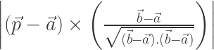
Step 5, especially the Euler angle part, is a little tricky. What is the rolling without slipping condition? We have but what is the magnitude of ? Well, we know what that is in terms of the Euler angles (and their time derivatives)!

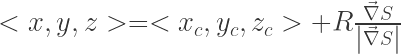
We could just grab their total amplitude, but we actually know something about the direction of . We know that it’s perpendicular to both the normal vector to the surface and to the direction of rolling.

Note that “the direction of rolling” is parallel to both the direction that the contact point is moving and the direction the center of the ball is moving, but you’ll see in a second that it’s much easier to use the ball for this (we’re normalizing that vector either way, so it doesn’t matter that they aren’t the same length, it only matters that they’re parallel). Out front, the magnitude of can be found from our simple rolling-without-slipping condition. Putting it all together yields:

Here’s how all that looks in Mathematica:

One thing that took me a while was figuring out how to make a ball look like it was rolling in Mathematica. Here’s how I did that:

Once you have the prototype ball you just use GeometricTransformation[ball[[1]], {m, r}] on it where m is the Euler rotation matrices dotted together and r is the location of the center of the ball.

Whoo hoo! On to step 6:

Here’s a comparison of 4 balls rolling on the function f(x,y)=sin(x)+sin(y) (it looks somewhat like an egg carton). They’re all started at the same point. Two are small and two are larger. In each size one is a solid ball and one is a shell. They all have the same mass:

And here’s the biggest ball I could get to roll on that surface. Why would there be a limit? Because you can’t use a ball that has a larger radius than the concave up radius of curvature at any point on its journey (Mathematica actually craps out right when this happens):

Here’s a still frame zoomed in a little showing that biggest ball right at the smallest radius of curvature:

One cool thing is that I can have Mathematica calculate the radius of curvature at all points along the trajectory. Here’s that plot where the red horizontal line is the radius of the ball:

How do you calculate the radius? You get it from this equation from way at the top of this post:

Note that before I really got my head wrapped around how to do this I thought I would have to calculate that radius of curvature (which, by the way depends on both where you are on the surface and what direction you’re rolling) directly from the definition of the curve itself. That was an interesting rabbit hole that this approach didn’t need (sorry for bothering you, my friend (and occasional guest blogger Art) for how to do this).

Your thoughts?

I’m really excited about this new type of modeling I can do. What are your thoughts? Here are some starters for you:

1. This is cool! What I especially like is . . .
2. This is dumb. I could do this on a napkin.
3. Why do you sometimes use hypens and sometimes not in the phrase ro-lli-ng—-wit-hou—-t-sli–ppin———-g?
4. Can you model a ball rolling on a rotating turntable? (actually this is what started all of this, I just haven’t gotten back to it yet)
5. What is up with that [[1]] you have to add to the GeometricTransformation command?
6. Will this make you a better golfer?
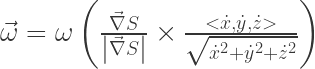
7. I like your handwriting better than . Do that from now on.
8. I hate your handwriting.
9. That level curve method is exactly what you did in 2D too, idiot.
10. This is Art: Are you telling me you didn’t use any of those calculations I gave you?!
11. What happens if the surface changes with time?

Situations that share equations of motion

Recently my friend Rhett Allain has been making some awesome videos showing how to solve complex problems with a Lagrangian approach. I love it when he posts a new video because it usually motivates me to try to model something similar.

Here’s the video he posted that inspired this post:

Rhett’s vid about two masses tied together through a hole in a table

I love this particular problem so I decided to dig in and see what I could learn from building my own model of it. One thing I was curious about was whether using a Lagrange multiplier technique could save me time. Basically I wondered if I could just model the two balls quite simply using Cartesian coordinates (xyz coordinates) and then directly imposing a constraint on the length of the string between them.

Unfortunately my first attempt had a huge mistake in it leading me to make an erroneous claim in this response video:

My initial video response to Rhett that has a big mistake in it (can you spot it?)

I got so excited that I had found an analogous system that shared the equations of motion, only upon reflection I realized I’d made a big mistake.

The length of the string should be given by the length above the hole:

along with the length of the string below the hole:

My mistake was assuming that was equivalent to:

Do you see the mistake? I hope it takes you more than a second or two to see it because I spent half a day thinking I’d discovered something really cool! Note that I still wrote this post so, trust me, there is still something cool, just not what I thought it was!

So what was I thinking? Well, let’s look at the code:

First let’s assume the masses are the same. Then the kinetic energy (the line starting with “T=”) would just be the kinetic energy of a free particle. In other words this would be just the model of a ball flying through a simple gravitational field. But that then gets corrected with the constraint line (the one that starts “cons = “). That says that the sum of squares of the variables needs to be a constant. That would imply that the particle has to stay on (or inside of) the surface of a sphere.

That’s what I got excited about in my video, because it seemed like the problem of the two balls connected through a hole with string was identical in form to a ball that has to stay on a sphere in a gravitational field. In hindsight I realize that a better way to describe that latter analogous problem is to call it what it is: a 3D pendulum!

But, ugh, I got the constraint wrong. It should have been that the length of string (which is held constant) is given by:

Of course in my case I put the hole at z=0 with “up” representing positive z’s. In other words the z in this problem will always be negative. So that gives:

Making that correction to the “cons = ” line gives me the correct model of the two particles tied together by a string running through that hole.

Now, here’s the cool part. If you set the masses equal, you can interpret the kinetic and potential energies (along with the constraint) to be describing a system where a ball has to stay on a surface described by that constraint.

Here’s what that looks like side by side:

See. I told you. Cool!

Your thoughts?

So what do you think? Here are some starters for you:

1. This IS cool. What I especially liked was . . .
2. Um, this isn’t cool, thanks for wasting my time. What I especially disapprove of is . . .
3. Let me get this straight: in an effort to look smart you posted a youtube vid that has a huge error in it and still thought you might as well post that mistake-ridden vid in this post. Loser.
4. This is Rhett. You’re awesome.
5. This is Rhett. Stop stalking me.
6. Why do you use the Lagrange multiplier approach? Are you afraid to type sines and cosines or something?
7. Lots of systems share a set of equations of motion. Why do you think it’s cool?
8. It took me exactly 2.3 seconds to find your dumb mistake.

Rigid bodies, formulation and examples

My friend Rhett Allain gave me a good challenge recently with this tweet:

What about a bead on a freely rotating hoop that can rotate in three dimensions?

— Rhett Allain (@rjallain) November 23, 2022

I had been working on a problem that he posted about regarding a bead sliding freely on a hoop that is spinning about an axis in its plane that goes through the center. That’s a pretty typical Lagrangian Dynamics-type problem and I wondered what would happen if the hoop wasn’t driven to constantly go with a particular angular frequency but rather was set spinning on that axis with that initial angular frequency but after that it would respond dynamically (speed up or slow down its rate of spinning) according to the physics involved. Here’s what that looks like:

But then when Rhett asked about letting the hoop be even more free to rotate, in other words not just around that one axis, I realized I’d have to calculate things a different way.

That led me to remind myself how to do Lagrangian Dynamics with rigid bodies, mostly dealing with things like the Inertia Tensor and body axes. This post is to make it so I don’t have to start from scratch with that again. Note that this post lays out the broad strokes of what I’m doing here.

Lagrangian dynamics with rigid bodies

For those of you hoping I’ll derive the Euler rotation equations, I should let you know that I don’t explicitly do that here. I get close, but I really move in a direction where I can solve the equations of motion and make some fun vids of the motion.

Here’s the steps involved:

1. Determine the generalized coordinates
2. Determine the kinetic and potential energies
3. Use the Principal Axes (actually you don’t have to do that)
4. Do all the usual Lagrangian stuff

Generalized coordinates (Euler rotations)

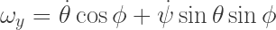
If you need to describe the orientation of a rigid body, how would you do it? I’ve done this with my students by asking them to all grab their chairs and figure out a systematic way to orient them the way mine is (which I do when they have their eyes closed). At first students think you just need the polar angles and because they figure that all the r’s are fixed and so you don’t need that third polar coordinate. But then I show them two situations with my chair that share the polar angles but look different. Ultimately my students usually land on a version of the Euler angles, which are really just the polar angles with a final twist of the body around the original vertical axis. Most texts call that last angle .

Well, if the Euler angles are the information that you need to describe the orientation of a rigid body, that means they’re just the perfect generalized coordinates for a Lagrangian Dynamics approach. All we have to be able to do is describe the potential and kinetic energy of the object as functions of the Euler angles and we’re good to go!

Kinetic and Potential energy as functions of the Euler angles

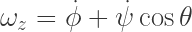
Early on physics students learn that if they’re dealing with rotating bodies they can replace with . Essentially what happens is that you realize that all parts of the system share an angular speed () even if different parts are traveling with different linear speeds (v). Since they all share the same thing, you can pull that out of any sums or integrals you’re doing to add up all the kinetic energy and whatever’s left you just lump into something we call the moment of inertia ().

The problem is that for oddly shaped things that simple approach doesn’t quite work. Sure all the pieces and parts still share an angular velocity (now we’re talking about the vector since the axis of rotation is something we need to know), but it’s not as simple as . Probably the easiest way to see that is that the angular momentum is not necessarily parallel to the angular velocity (STOP: read that again, as it’s one of the single most important aspects of rigid body motion and it sounds really weird to most people). Instead there’s a relationship between the angular momentum vector and the angular velocity vector that’s more complicated. If you know the angular velocity you can find the angular momentum with a 3D rotation, and that’s done computationally with a 3×3 tensor which we call the inertia tensor. Then you have . Essentially a 3×3 tensor dotted into a vector gives you a new vector that (often) points in a new direction (hence them not being parallel anymore).

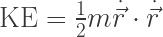
Really the inertia tensor has just what we need. Just like we can do for kinetic energy normally (try it!), we can do or:

Aha! So now if we know how both the inertia tensor and the angular velocity vector can be described by the Euler angles (and their time derivatives) we’re in business!

The inertia tensor is certainly calculate-able if you know the orientation of the object (which you do if you know the Euler angles). Essentially you can figure out where all the particles of the body are and then do all the integrals necessary for the inertia tensor (remember, the tensor is just made up of what’s left after you factor out the common terms that all the particles share – namely the angular velocity – so it’s just a collection of sums/integrals involving the locations of the particles). What really sucks, though, is that at every point in time there is a new orientation and hence a whole new set of integrals to do. Ugh. Don’t worry though, that gets a lot easier in the next section!

The angular velocity is certainly a function of the time derivatives of the Euler angles since as they change they rotate the body, and rotation is all that angular velocity is used to describe. Here’s the cool part: the angular velocity () is equal to the sum of three vectors, one for each Euler angle. Each Euler angle contributes it’s time derivative (which is exactly the right units for angular velocity) in the direction of the instantaneous axis of rotation that Euler angle rotates around. I know, that was complicated, but it’s relatively straightforward to work out:

First consider the easiest one: . When you think about it that polar vector, all it does is rotate everything around the vertical-, or z-, axis. Therefore ‘s contribution to is .

Next consider : When it changes, it tilts the object further from the vertical. But it does so in the plane determined by . The instantaneous axis of rotation is the location of the new y-axis after the rotation. So that means that the contribution to is

Finally we have . It rotates the body around its original vertical axis. That means its instantaneous axis of rotation is wherever its vertical axis has gotten to after the polar angles have done their thing. So ‘s contribution is .

All together then we have these for the components of the angular velocity vector:

Only calculate the inertia tensor once!

Ok, we have the angular velocity all set to go, but we saw how the inertia tensor, while definitely a function of the Euler angles, might have to be calculated over and over again. What if we only had to do it once!

The trick is to decide to think about how things feel in the frame of the rigid body. In what we call the “body-frame” it sits there while the world moves around it. Specifically the angular velocity vector is all over the place. But, and this is the important part, the inertia tensor is fixed! You just have to calculate it once in that orientation. So the problem becomes determining what the angular velocity vector (which we calculated above) looks like in that body-frame.

But luckily the Euler angles were built to transform any vector into a new rotated state. So we just need to apply the Euler rules to the angular velocity vector above. Except that we’re trying to describe how things look to the body frame, so what we really need is the reverse of the Euler rules, namely:

• negative rotation of around the z-axis, followed by. . .
• a negative rotation of around the y-zaxis, followed by . . .
• a negative rotation of around the z-axis

I know, that seems weird, but, trust me, it does the trick. All of those rotations are pretty straightforward for something like Mathematica to do so we’re in business: Calculate the inertia tensor once, figure out the lab-based angular velocity vector, and then do the steps above to find the body-frame version of the angular velocity vector. Then you calculate the kinetic energy.

Here’s what that looks like in Mathematica:

After the “KE=…” line is the usual construction of how I do Lagrangian Mechanics. The “Method->…” stuff was suggested by Mathematica after the first solve seemed to fail. That Method fix did the trick.

You’ll note that my inertia tensor (“Ithing”) is really simple. There are no off-diagonal terms in the matrix because I wanted to investigate the same sort of thing I did in this post about flipping handles in space. The section below called “Principal Axes frame” is how I teach my students to find the magical orientiation of an object where its inertia tensor has that simple setup. Note that it’s not necessary for the work I’ve laid out here.

Note that while this makes it pretty do-able, you’re still going to want a Computer Algebra System to help. Here’s just the Euler-Lagrange equation (all of this equals zero) for a generic inertia tensor:

Putting it to use to answer Rhett

Ok, so now I had the tools to answer Rhett’s question. I’ve got an interesting system made up of a hoop and a bead. What I decided to do was to fix for the hoop at zero because otherwise I would have to keep track of the bead’s sliding separate from the rotation of the hoop around it’s (original) vertical axis. The orientation of the hoop when all the Euler angles are zero is horizontal. 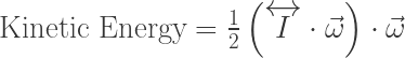So I first set to to stand it up and then I set to some initial spin rate.

For the bead I just determine it’s contribution to the inertia tensor of the system. Luckily that’s just a simple function of (remember I fix that at zero for the hoop). So I basically do the same thing as before. Here’s the Mathematica:

Really I have to carefully do the hoop and the bead separately when doing the calculations, but otherwise it’s similar to what I did above.

Here’s the results!

You can see how the hoop starts to tilt over. It has to to maintain a constant angular momentum (since there’s no torque in the problem if you don’t fix the axis of the hoop).

Principal Axes frame

I noted above that you don’t have to use the principal axes frame but I wanted to put this in for my future self:

When I teach this I point out how difficult things are when the angular moment is not parallel to the angular velocity. I ask them if they’d like it if we could make that disappear. Usually they say yes.

I tell them that there are some magic scenarios when the two are parallel. Essentially there are three axes that if you rotate around them you get an angular momentum in that same direction. There are a few ways to figure them out, but most are either difficult to understand mathematically (eigenvectors of the inertia tensor) or would take forever (just spin the object along all possible axes and look to see when the angular momentum is along that same axis). But there’s one way I’ve found that my students can do. I have to explain how a diagonalized inertia tensor does the trick. I do that by saying that we’ll just keep orienting the object until we find that all three of the magic axes are along the normal lab axes (x-, y-, and z-axes). In that orientation, you get what we need as long as there are no non-zero off-diagonal components of the inertia tensor.

So I provide my students with a Mathematica document that lets them freely adjust the Euler angles for an object and it constantly recalculates the inertia tensor for that orientation (see the last section above to understand why the tensor changes with orientation). What’s cool is that they can see how certain adjustments to the Euler angles tends to reduce at least one of the 3 off-diagonal components and they usually quickly find a systematic way to get them all to be vanishingly small. When they do that, they’re staring at the orientation that puts the magic axes along the lab axes!

Your thoughts?

I’d love to hear what you think. Here are some starters for you:

• I love this! What I especially am surprised by is . . .
• This is dumb. I especially hated . . .
• So whatever Rhett says you just do? That sounds interesting . . .
• Once again no python, loser
• I thought you only had a chromebook at home. How are you doing all this Mathematica?
• Whoa, it looks like you do the rotation first in your Mathematica code. Didn’t you say it comes last?
• Wait, I don’t have to diagonalize the inertia tensor before doing these kinds of simulations? That’s so cool!
• Do you provide tools to help your students unbolt their chairs from the desks?
• I want to hear more about how students can systematically find the principal axes by just adjusting the Euler angles!
• Why don’t you have to do the normal accelerated frame adjustments for your kinetic energy? (it’s quite late as I type this and I realize I don’t have a good answer beyond “it just works”)